Here, you’ll find a H2 Math crash course on the topics learned in JC1.
Topics Covered in H2 Math
Here are H2 Math Topics that typically covered in JC1. There’s some slight variations among different schools, but theses are the topics most schools cover in JC1:
- System of linear equations
- Inequalities
- Curve sketching
- Transformation of graphs
- Functions
- Vectors
- Differentiation Techniques
- Application of differentiation
- Integration
- Application of Integration
- Maclaurin’s Expansion
- Differential Equations
- Sequences and Series + Summation Notation
- Arithmetic Progression and Geometric Progression (AP&GP)
Click on the link to each of the topic above to go to the quick crash course on the topic.
System of Linear Equations
Systems of linear equation is often the first chapter that is learned in H2 Math in JC1.
A system of linear equations consist of 2 or more linear equations. Linear equations are equations where the unknown variable has a power of 1. Questions from this chapter often involves solving a system of linear equation with 3 or 4 unknowns.
Here’s an example of a system of linear equation:
3x+y-z=5
2x+y+z=2
x-2y+2z=1
The solution for this system of linear equation is: x = 11/7, y= -3/7, z = -5/7
The use of the graphic calculator (APPS –> Polysmlt) is used to solve the questions. –> Go here to learn step-by-step on how to use GC to solve systems of linear equation.
Note that in order to solve for n unknowns, you’ll need n equations.
Inequalities
There are 2 ways to solve inequalities:
- without calculator (i.e. mathematically)
- graphically using the graphic calculator (G.C)
Solving Inequalities without the calculator
Before you move on to the inequality, make sure you are familiar with the rules of inequalities, and also how to solve quadratic inequalities (you’ve learned this in O Level Additional Math). Once you are familiar with these topics learned in secondary school, here are the new concepts that you’ll learn:
- Solve polynomial inequalities –> step-by-step tutorial here
- Solve inequalities with polynomial fractions –> step-by-step tutorial here
- Solve inequalities containing quadratic functions that are always positive or negative –> step-by-step tutorial here
- Solve inequalities with modulus signs –> step-by-step tutorial here
Solving Inequalities graphically using the G.C
This involves using the graph function on the graphic calculator, and determine which range of values of x satisfy the inequality. Read here for detailed explanation.
Curve Sketching
In curve sketching, you’ll need to use the graphic calculator A LOT, to sketch the graph. You’ll be tested on sketching graphs written in cartesian form (i.e. y in term of x, or x in terms of y), as well as parametric form (i.e. y in terms of a parameter e.g. p, and x in terms of the same parameter e.g. p)
Curves to Sketch in Cartesian Form
You are expected to use the graphic calculator to sketch these graphs. Click on the link below to see step-by-step tutorial on how to sketch these graphs using the graphic calculator.
- Circles: (x-a)² +(y-b)² = r²
- Ellipses: (x-a)²/c² +(y-b)²/d² = 1
- Hyperbolas
- Rectangular Hyperbolas: y= (ax+b)/(cx+d)
- y= (ax²+bx+c)/(dx+c)
Sketching curves written in parametric form
A parametric equation is one in which a few quantities are expressed as a function of a parameter.
This is an example of a parametric equation:
y = cos t; x= sin t
Transformation of graphs
In this chapter, we learn how to transform (scale, translate, reflect, etc.) these graphs from y = f(x):
Read here where I explain how to do each type of transformation.
The H2 A Level exam often tests students on multiple transformations. Learn how to do multiple transformations, and the recommended order here.
Functions
In the function chapter, students learn what functions are and then apply them to :
- finding the range / domain of functions
- what is one-one function
- inverse functions
- condition for them to exist (i.e. they have to be one-one)
- finding range/ domain of inverse functions
- finding the rule of an inverse function
- composite functions
- condition for composite functions to exist
- finding range/ domain of composite functions
- finding the rule of a composite function
You’ll find the detailed notes on this chapter on functions here.
Vectors
In H2 Math, vectors is a (very) long chapter. I’ll recommend looking at points below, and testing yourself what’s the concept behind them, and then click on the link below, to bring you to a detailed explanation on each vector concept in your H2 A Level Math:
- what are vectors
- what’s a position vector vs a direction vector
- how to denote vectors
- magnitude of vectors
- unit vectors
- parallel vectors
- collinear
- ratio theorem
- scalar product
- vector product
- equation of lines
- equation of planes
- length of projection
- perpendicular distance
Differentiation Techniques
Properties of differentiation
In differentiation techniques, you should be familiar with the different differentiation techniques:
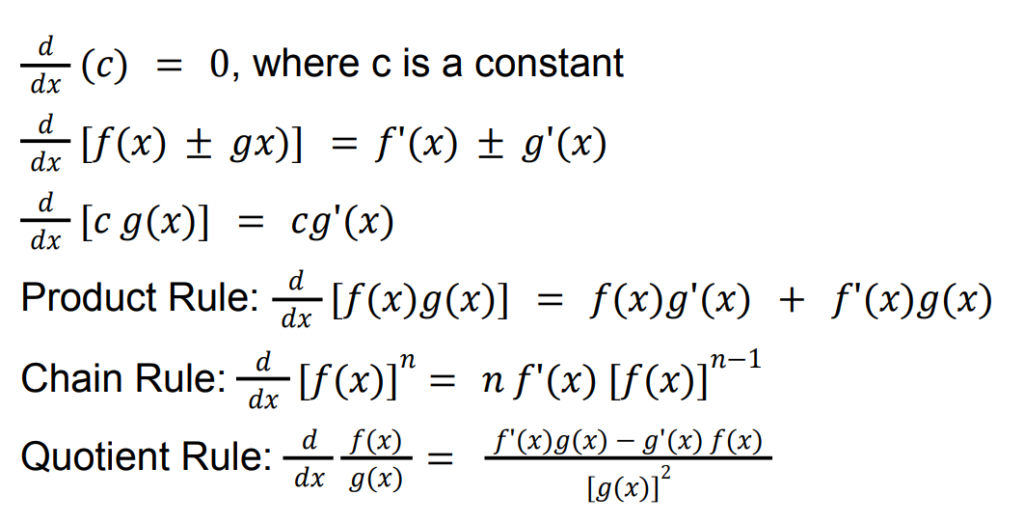
Differentiation Formulae tested in H2 A Level Math
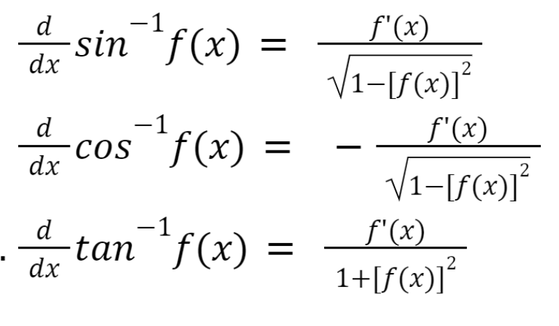
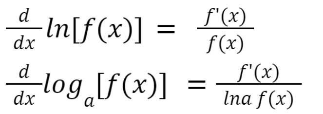
Once you are familiar with those properties of differentiation, and applying chain rule, product rule, quotient rule and so on, it’s time to be familiar with the differentiation formulae that you learn:
Differentiation of Algebraic Functions

Differentiation of Trigonometric Functions
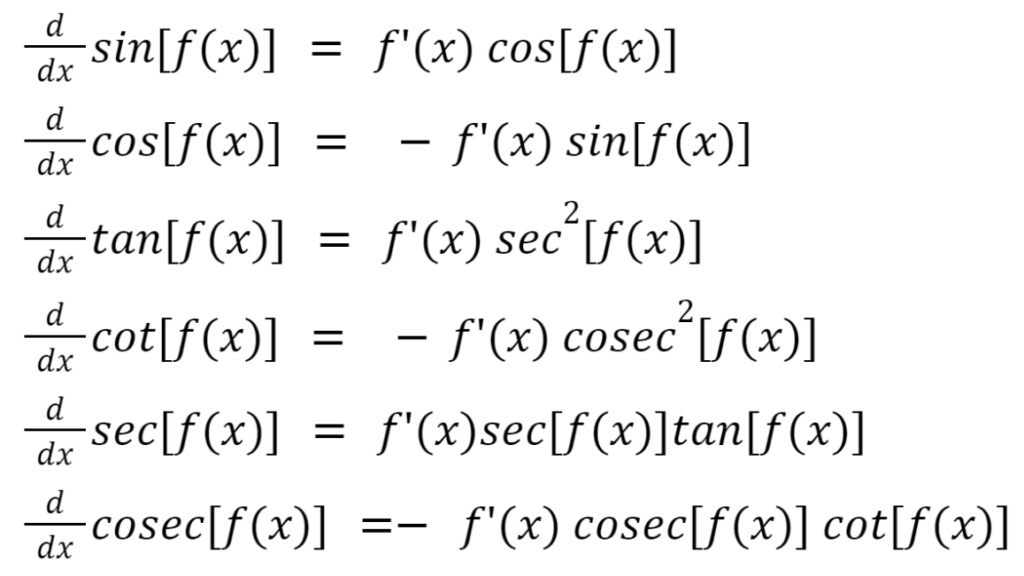
Differentiation of Inverse Trigonometric Functions
Differentiation of exponential functions

Differentiation of logarithmic functions
Differentiation of parametric equations
A parametric equation is one in which a few quantities are expressed as a function of a parameter.
This is an example of a parametric equation:
y = cos t; x= sin t
To differentiate a parametric equation, you’ll need to find dy/dt and dx/dt. dy/dx = (dy/dt) /(dx/dt)
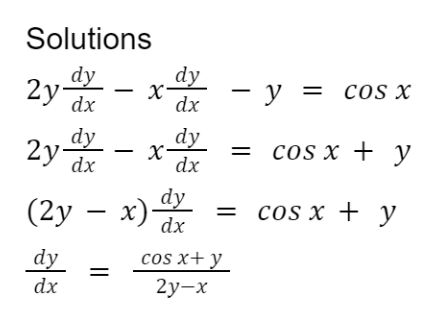
Implicit Differentiation
Implicit differentiation is used when we do not have an equation expressed as y in terms of x. When that happens, we use implicit differentiation.
The following is an example of obtaining dy/dx by implicit differentiation:

Application of Differentiation
Application of differentiation is a chapter that is very like your A Level Additional Math, just with more added complexity, and with the new formulae you learn at A levels.
In this topic, you learn be tested on:
- increasing and decreasing functions
- finding maximum and minimum point
- application of differentiation to tangents and normals
- application of differentiation to maximum and minimum problems
- application of differentiation to rate of change (using chain rule)
I explain in the details the above concepts here.
Integration
Integration at A Level is a huge step from O Level integration. Suddenly, you have way more different ways you can integrate, and you’ll often, it involves trigonometric manipulation (example: 2023 H2 A Level Paper 1 Question 4 integration question ).
In this topic on integration, you’ll need to be familiar with the properties of integration, and all the formulae. I’ve summarized all of them here. Then you’ll need to use your observing eyes to determine which method to use. This comes from experience — i.e. conscious pratice.
Application of Integration
In this section, you’ll apply integration to finding:
Maclaurin’s Expansion
Maclaurin’s expansion can be used to approximate a function, f(x) into a polynomial form. The approximation can be done using this formula here:

This formula is given in the formula booklet during your A Level Exam, and does not need to be memorized.
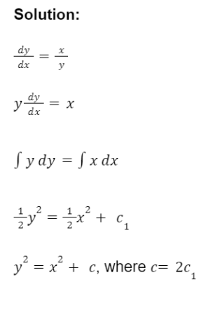
Differential Equations
In H2 A Level Math, you are given an equation with dy/dx, y and x, and asked to find y. This is known as a first-order differential equation, and you are to find an expression for y in terms of x using the variable separable method.
Below is an example of solving a differential equation:

Sequences and Series + Summation Notation
I’ve broken down this chapter on sequences and series into many different parts. Click on the link to learn about each concept:
- Sequences and series
- Summation: Introduction
- Finding summation using the graphic calculator
- Method of difference and summation
Arithmetic Progression and Geometric Progression (AP&GP)
Arithmetic Progression
An arithmetic progression is one in which each consecutive term differs by a common difference, d.
If the first term of an arithmetic progression is a, and the common difference is d, then
- nth term = a + (n-1)d
- sum of first n terms = 1/2 n[2a+(n-1)d] = 1/2 n [a + nth term]
Geometric Progression (GP)
A geometric progression is one in the ratio of 2 consecutive terms is a constant, r.
r = (nth term)/ ((n+1)th term)
If the first term of a geometric progression is a, and the common ratio is r, then
nth term of the geometric progression = arⁿ⁻¹

For a geometric progression (GP), the sum to infinity exists or the GP is convergent if |r| <1. If that happens, the sum to infinity can be found be the formula:

Hope this crash course on JC1 H2 A Level Math is useful to you! =)
All the notes for H2 A Level Math
Go here to find all the notes and resources for H2 A level Math.
